We illustrate the process law feature on a simple deterministic problem, without discrete modes. We consider a classical 2D integrator
\(\displaystyle
\left \lbrace
\begin{array}{l}
\min \frac{1}{2}\int_0^T (u_1(t)^2 +u_2(t)^2)dt \ +\ ((x_1(T)-x_2(T))^2\\
\dot x_1 = u_1(t)\ ,\ \dot x_2 = u_2(t)\\
u_1, u_2, x_1, x_2\in[-1, 1]\\
T = 1.
\end{array}
\right .
\)
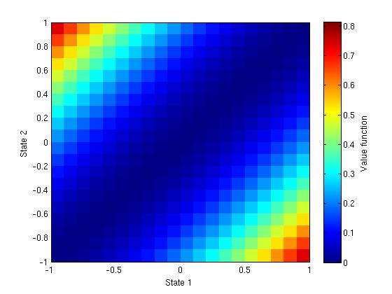
The figure shows the value function at initial time. As expected, the value function is 0 along the first bisector (x1 = x2) and increases symmetrically when getting farther form it.
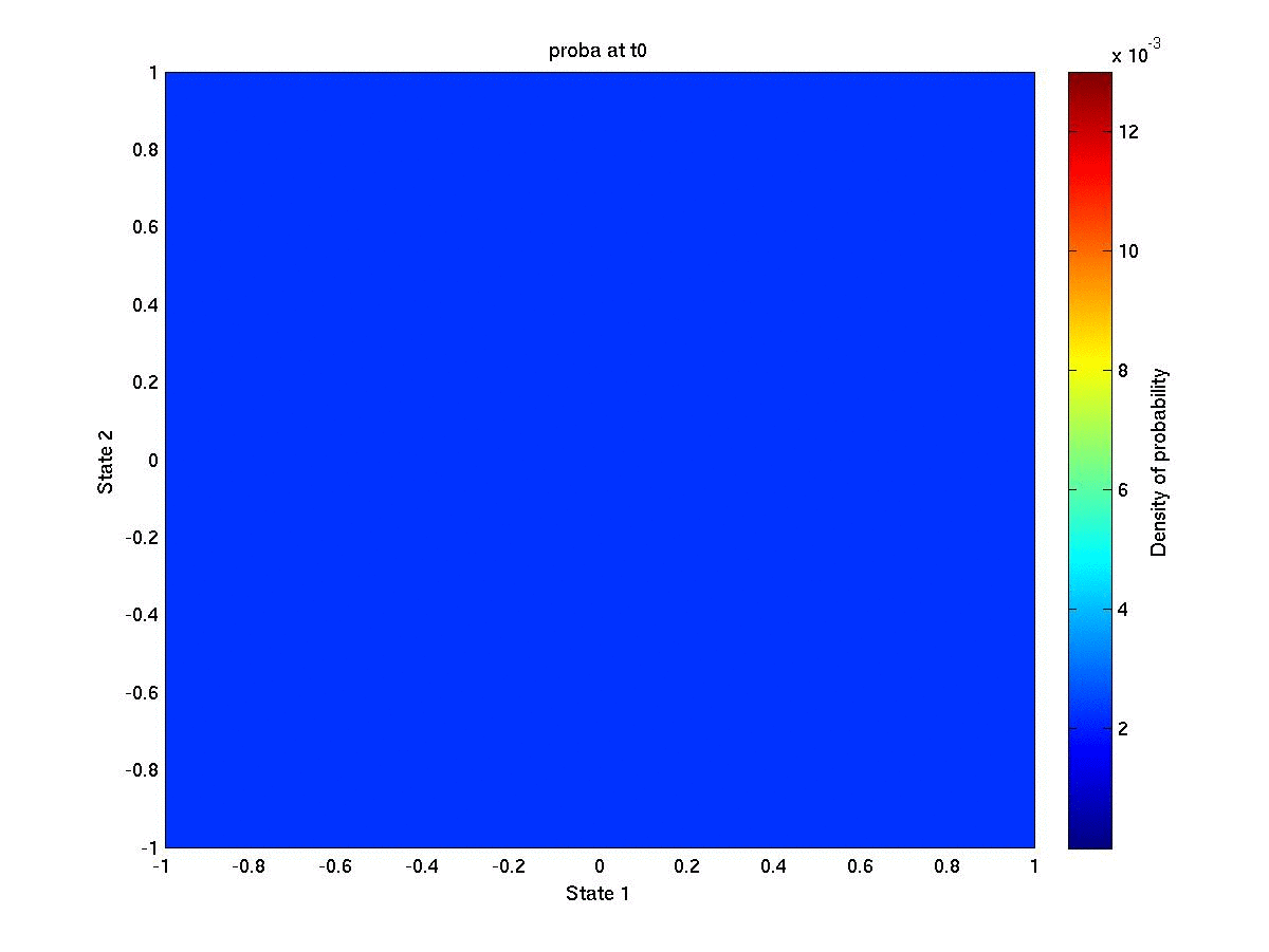
We set the state probabilities at initial time according to a discrete uniform distribution
\(\displaystyle\mathcal{P}_0(x_i)_{i=1, \ldots, N_{grid}} = \frac{1}{N_{grid}}\)
The following animated figure shows the evolution of the state probabilities over the grid for each time step. We observe a concentration of the distribution towards the first bisector. This is not surprising since every optimal trajectory tries to reach the bisector with minimal quadratic cost.